Tutorial 4: Mode shapes
Goal: look at what each mode does, three ways: a static chart of the participating degrees of freedom, an interactive 3-D view of the deformed turbine, and an animation for VTK viewers.
Script: examples/04_mode_shapes.py · Data: one synthetic operating point
at 8 m/s (see The synthetic turbine) · Run time: seconds
The code
from vane.io import mbc3_transform, read_lin_file
from vane.modal import label_solution, modes_from_mbc
from vane.viz import (
    deform_mode,
    plot_mode_3d,
    plot_mode_fowt,
    plot_mode_participation,
    write_mode_animation_vtk,
)

WIND_SPEED = 8.0  # m/s
def main(argv: list[str] | None = None) -> int:
    """Run the tutorial.

    Parameters
    ----------
    argv : list[str] or None, optional
        Command-line arguments; ``None`` reads ``sys.argv``.

    Returns
    -------
    int
        The exit status.
    """
    args = output_parser(__doc__).parse_args(argv)
    with output_directories(args.output) as (data, figures):
        # 1. One operating point, its modes and their labels.
        paths = SyntheticTurbine().write_operating_point(data / "lin", WIND_SPEED)
        solution = modes_from_mbc(mbc3_transform([read_lin_file(p) for p in paths]))
        labels = label_solution(solution)
        for k, label in enumerate(labels):
            frequency = solution.natural_frequencies_hz[k]
            print(f"mode {k}: {frequency:.4f} Hz  {label.label}")
        tower = next(k for k, lab in enumerate(labels) if "Fore-Aft" in lab.label)
        flap = next(k for k, lab in enumerate(labels) if "Regressive" in lab.label)

        # 2. Static participation charts of two modes. Short names label the bars
        # with the degree of freedom and, after MBC3, its multi-blade coordinate
        # (collective, cosine or sine) rather than blades 1, 2 and 3.
        with figure_style():
            figure, axes = plt.subplots(2, 1, figsize=(17.0 / 2.54, 4.4))
            for ax, k in zip(axes, (tower, flap), strict=True):
                plot_mode_participation(solution, k, top_n=4, ax=ax, short_names=True)
                frequency = solution.natural_frequencies_hz[k]
                ax.set_title(f"{labels[k].label}, {frequency:.3f} Hz")
            figure.tight_layout()
            save_figure(figure, figures / "tutorial_mode_participation.png")

        # 3. Interactive 3-D views (open the HTML files in a browser).
        for k in (tower, flap):
            plot_mode_fowt(solution, k).write_html(data / f"mode_{k}_turbine.html")
            plot_mode_3d(solution, k).write_html(data / f"mode_{k}_phasors.html")
        print(f"3-D views written: mode_{tower}_*.html, mode_{flap}_*.html")

        # 4. A VTK animation of the regressive flap mode.
        deformation = deform_mode(solution, flap)
        members = deformation.geometry.members
        points = np.vstack([member.nodes for member in members])
        displacement = np.vstack(deformation.displacements)
        lines, start = [], 0
        for member in members:
            count = len(member.nodes)
            lines.append(list(range(start, start + count)))
            start += count
        written = write_mode_animation_vtk(
            points, displacement, data / "regressive_flap.pvd", lines=lines
        )
        frames = [path for path in written if path.suffix == ".vtk"]
        print(
            f"VTK animation: regressive_flap.pvd and {len(frames)} frames, "
            f"{points.shape[0]} nodes on {len(members)} members"
        )
    return 0
Run it
$ python examples/04_mode_shapes.py --output shapes
mode 0: 0.3000 Hz  1st Tower Side-Side
mode 1: 0.3215 Hz  1st Tower Fore-Aft
mode 2: 0.5564 Hz  1st Blade Flap (Regressive)
mode 3: 0.7133 Hz  1st Blade Flap (Collective)
mode 4: 0.8590 Hz  1st Blade Flap (Progressive)
Figure written: tutorial_mode_participation.png
3-D views written: mode_1_*.html, mode_2_*.html
VTK animation: regressive_flap.pvd and 24 frames, 89 nodes on 7 members
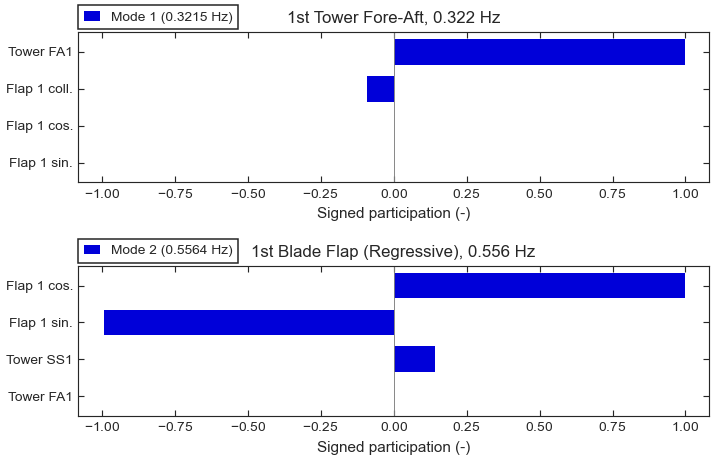
Signed participation of the four most active degrees of freedom in the tower fore-aft mode (top) and the regressive flap mode (bottom).
Step by step
1. The modes. The script repeats the analysis of Tutorial 2: MBC3 transform and eigenanalysis and the labels of Tutorial 3: Mode identification and the Campbell diagram at 8 m/s, and picks the tower fore-aft and the regressive flap modes by their labels.
2. Participation charts. plot_mode_participation()
draws the most active degrees of freedom of one mode as bars, signed by their phase
relative to the dominant one: a negative bar moves in opposition. The tower fore-aft
mode is almost pure tower motion, with the collective flap moving against it at a tenth
of its amplitude. In the regressive mode the cosine and sine flap coordinates have equal
size and a phase difference: the rotor disc wobbles, which in the fixed frame is the
backward whirl. With short_names=True the chart labels each bar with a short
degree-of-freedom name and, after the MBC3 transform, its multi-blade coordinate:
the three blade rows are the collective, cosine and sine coordinates, not blades 1, 2
and 3. The figure is drawn inside vane.viz.plot_style(), the plotting style of
VANE’s static figures.
3. Interactive views. plot_mode_fowt() deforms a
schematic bottom-fixed turbine by the mode shape and returns a
Plotly figure; plot_mode_3d() draws the complex mode
shape as phasors. The script writes both as HTML files to open in a browser. The
geometry is inferred from the degrees of freedom of the solution (a bottom-fixed
turbine here, since there are no platform states); pass a
FowtGeometry for the dimensions of a specific
turbine.
4. A VTK animation. deform_mode() returns the
same deformation as complex nodal displacements on each member of the geometry. The
script stacks the members into one point set, with one polyline per member, and
write_mode_animation_vtk() writes 24 frames over one period
of the oscillation as legacy VTK files, tied together by regressive_flap.pvd. Open
the .pvd file in a VTK viewer and press play to see the rotor disc whirl. For a single
frozen shape, use write_mode_shape_vtk().
Exercises
Plot the collective flap mode (
mode 3) and compare it with the regressive one: the three blades now move in phase, and the tower fore-aft motion appears.Call
plot_mode_fowt(solution, k, phase_deg=90.0)to freeze the regressive mode a quarter period later, and see the deformation move from the cosine to the sine pattern.
See Visualization for every plotting function and its options. Next: Tutorial 5: Azimuth averaging and its error.