Tutorial 2: MBC3 transform and eigenanalysis
Goal: read the .lin files of one operating point, transform the rotating blade
states into the fixed frame and average over azimuth with
mbc3_transform(), then find the natural frequencies,
damping ratios and participation of the modes with
modes_from_mbc().
Script: examples/02_mbc_and_eigenanalysis.py · Data: one synthetic
operating point (see The synthetic turbine) · Run time: seconds
The code
from vane.io import mbc3_transform, read_lin_file
from vane.modal import (
    azimuth_spread,
    compute_modes,
    modes_from_mbc,
    participation_from_modes,
)

WIND_SPEED = 8.0  # m/s
N_AZIMUTHS = 12
def main(argv: list[str] | None = None) -> int:
    """Run the tutorial.

    Parameters
    ----------
    argv : list[str] or None, optional
        Command-line arguments; ``None`` reads ``sys.argv``.

    Returns
    -------
    int
        The exit status.
    """
    args = output_parser(__doc__).parse_args(argv)
    with output_directories(args.output) as (data, figures):
        # 1. Write one operating point: twelve azimuths over one revolution.
        turbine = SyntheticTurbine()
        paths = turbine.write_operating_point(
            data / "ws080", WIND_SPEED, n_azimuths=N_AZIMUTHS
        )

        # 2. Read the files.
        files = [read_lin_file(path) for path in paths]
        first = files[0]
        print(f"Read {len(files)} files, {paths[0].name} to {paths[-1].name}")
        print(
            f"  {first.n_x} states, {first.n_u} inputs, {first.n_y} outputs; "
            f"rotor speed {first.rotor_speed:.4f} rad/s, wind {first.wind_speed} m/s"
        )
        rotating = [
            d
            for d, r in zip(first.x.descriptions, first.x.rotating_frame, strict=True)
            if r
        ]
        print(f"  {len(rotating)} states in the rotating frame, e.g. {rotating[0]!r}")

        # 3. MBC3 transform and azimuth average.
        mbc = mbc3_transform(files, retain_per_azimuth=True)
        print()
        print("MBC3 transform")
        print(f"  performed: {mbc.performed_transformation}, blades: {mbc.n_blades}")
        print(f"  rotor speed {mbc.rotor_speed_rpm:.3f} rpm, wind {mbc.wind_speed} m/s")
        print(f"  azimuths (deg): {np.round(mbc.azimuths_deg, 1).tolist()}")
        print(f"  ndof2 = {mbc.ndof2}, ndof1 = {mbc.ndof1}")
        names = [
            short_name(desc, coord)
            for desc, coord in zip(
                mbc.state_descriptions[: mbc.ndof2],
                mbc.mbc_coordinates[: mbc.ndof2],
                strict=True,
            )
        ]
        print(f"  displacement states: {names}")

        # 4. Eigenanalysis of the averaged matrix.
        solution = modes_from_mbc(mbc)
        print()
        print(
            f"Eigenanalysis: {solution.n_modes} oscillatory modes, "
            f"{solution.n_rigid_body_modes} rigid-body DOF, "
            f"{solution.n_overdamped} real eigenvalues"
        )
        print("  mode   f_n (Hz)   f_d (Hz)   damping (-)")
        for k in range(solution.n_modes):
            print(
                f"  {k:4d}   {solution.natural_frequencies_hz[k]:8.4f}   "
                f"{solution.damped_frequencies_hz[k]:8.4f}   "
                f"{solution.damping_ratios[k]:10.4f}"
            )

        # 5. Participation of each degree of freedom in each mode.
        participation = participation_from_modes(solution)
        print()
        print("Participation (each column scaled to a maximum of 1)")
        print(
            "  DOF            "
            + "".join(f"  mode {k}" for k in range(solution.n_modes))
        )
        for row, name in enumerate(names):
            values = "".join(f"  {v:6.3f}" for v in participation.magnitude[row])
            print(f"  {name:<14}{values}")

        # 6. Per-azimuth spread left by the periodic (3P) content.
        spread = azimuth_spread(mbc)
        print()
        print("Azimuth spread of the natural frequency (Hz)")
        print("  " + ", ".join(f"{s:.2e}" for s in spread.natural_frequency_std))

        # 7. For comparison: one frozen-azimuth matrix in the mixed frame.
        assert first.a is not None
        frozen = compute_modes(first.a, ndof2=mbc.ndof2, ndof1=0)
        print()
        print("Frozen azimuth (0 deg), mixed frame, no MBC")
        print(
            "  f_n (Hz): "
            + ", ".join(f"{f:.4f}" for f in frozen.natural_frequencies_hz)
        )

        with figure_style():
            figure, (left, right) = plt.subplots(
                1, 2, figsize=(6.5, 4.0), gridspec_kw={"width_ratios": [1.0, 1.3]}
            )
            for x, freqs in (
                (0, frozen.natural_frequencies_hz),
                (1, solution.natural_frequencies_hz),
            ):
                left.hlines(freqs, x - 0.3, x + 0.3)
            left.set_xticks([0, 1], ["frozen\nazimuth", "MBC3\naverage"])
            left.set_xlim(-0.6, 1.6)
            left.set_ylabel("Natural frequency (Hz)")
            left.set_title("Frequencies")
            image = right.imshow(
                participation.magnitude, vmin=0.0, vmax=1.0, aspect="auto"
            )
            right.set_xticks(range(solution.n_modes))
            right.set_xlabel("Mode")
            right.set_yticks(range(len(names)), names)
            right.set_title("Participation")
            right.grid(visible=False)
            figure.colorbar(image, ax=right)
            figure.tight_layout()
            save_figure(figure, figures / "tutorial_mbc_modes.png")
    return 0
short_name (in the script) only turns a description such as
"ED 1st tower fore-aft bending mode DOF (internal DOF index = DOF_TFA1), m" into
TFA1 for the printed tables.
Run it
$ python examples/02_mbc_and_eigenanalysis.py
Read 12 files, ws080.1.lin to ws080.12.lin
  12 states, 2 inputs, 8 outputs; rotor speed 0.9587 rad/s, wind 8.0 m/s
  6 states in the rotating frame, e.g. 'ED 1st flapwise bending-mode DOF of blade 1 (internal DOF index = DOF_BF(1,1)), m'

MBC3 transform
  performed: True, blades: 3
  rotor speed 9.155 rpm, wind 8.0 m/s
  azimuths (deg): [0.0, 30.0, 60.0, 90.0, 120.0, 150.0, 180.0, 210.0, 240.0, 270.0, 300.0, 330.0]
  ndof2 = 6, ndof1 = 0
  displacement states: ['TFA1', 'TSS1', 'GeAz', 'BF1 collective', 'BF1 cosine', 'BF1 sine']

Eigenanalysis: 5 oscillatory modes, 1 rigid-body DOF, 1 real eigenvalues
  mode   f_n (Hz)   f_d (Hz)   damping (-)
     0     0.3000     0.3000       0.0097
     1     0.3215     0.3210       0.0589
     2     0.5564     0.5508       0.1415
     3     0.7133     0.7091       0.1089
     4     0.8590     0.8554       0.0921

Participation (each column scaled to a maximum of 1)
  DOF              mode 0  mode 1  mode 2  mode 3  mode 4
  TFA1             0.000   1.000   0.000   0.270   0.000
  TSS1             1.000   0.000   0.143   0.000   0.050
  GeAz             0.000   0.000   0.000   0.000   0.000
  BF1 collective   0.000   0.090   0.000   1.000   0.000
  BF1 cosine       0.014   0.000   1.000   0.000   0.998
  BF1 sine         0.058   0.000   0.992   0.000   1.000

Azimuth spread of the natural frequency (Hz)
  4.78e-14, 3.64e-03, 1.49e-14, 3.45e-05, 5.75e-15

Frozen azimuth (0 deg), mixed frame, no MBC
  f_n (Hz): 0.3002, 0.3266, 0.7069, 0.7080, 0.7134
Figure written: tutorial_mbc_modes.png
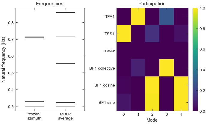
Left: the frozen-azimuth matrix has three blade frequencies near 0.71 Hz; the MBC3 average splits them into 0.556, 0.713 and 0.859 Hz. Right: the participation of each degree of freedom in each of the five modes.
Step by step
1. One operating point is a set of files. OpenFAST writes one .lin file per
linearization time, named <case>.<n>.lin. A CalcSteady linearization with
NLinTimes = 12 writes twelve snapshots spread over one rotor revolution, and
together they describe one operating point. The synthetic turbine writes the same
twelve files at 8 m/s and 9.155 rpm.
2. Reading. read_lin_file() returns a
LinFile with the header values (rotor_speed in rad/s,
azimuth in rad, wind_speed), the operating-point tables x, u and y
with their descriptions and rotating-frame flags, and the matrices a to d. The
six blade states carry the flag T: OpenFAST writes them in each blade’s rotating
frame.
3. The MBC3 transform. mbc3_transform() groups the
rotating states into blade triplets by their descriptions (blade 1, 2 and 3 of the
same degree of freedom), replaces each triplet by its collective, cosine and sine
coordinates, transforms the matrices of every azimuth into the fixed frame, and
averages them. It also reorders the states into the [q2, q2dot, q1] layout: here
six displacements, their six rates and no first-order states (ndof2 = 6,
ndof1 = 0). The descriptions of the three transformed flap states still name blades
1, 2 and 3; mbc.mbc_coordinates says which is the collective, cosine and sine
coordinate. retain_per_azimuth=True keeps the transformed matrix of each azimuth,
which step 6 needs.
4. The eigenanalysis. modes_from_mbc() solves the
eigenvalue problem of the averaged matrix and keeps one eigenvalue per complex
conjugate pair, sorted by frequency. Two degrees of freedom have no oscillatory mode:
the generator azimuth has a zero eigenvalue (counted as a rigid-body degree of
freedom), and the rotor speed decays without oscillating (one real eigenvalue,
n_overdamped). Five modes remain: tower side-side at 0.300 Hz, tower fore-aft at
0.3215 Hz, and three flap modes at 0.556, 0.713 and 0.859 Hz.
Check the flap modes by hand. In the rotating frame each blade’s flap frequency is \(f_r=\sqrt{0.68^2+1.6\,f_\Omega^2}\), with the rotor frequency \(f_\Omega = 9.155/60 = 0.1526\) Hz, so \(f_r = 0.7069\) Hz. Seen from the fixed frame, a backward-whirling (regressive) flap motion appears at \(f_r - f_\Omega = 0.554\) Hz and a forward-whirling (progressive) one at \(f_r + f_\Omega = 0.860\) Hz, while the collective mode stays near \(f_r\). The computed 0.556, 0.713 and 0.859 Hz differ from these estimates only by the coupling to the tower.
5. Participation. participation_from_modes()
measures how strongly each degree of freedom takes part in each mode, from the
magnitudes of the mode shape, with each column scaled to a maximum of 1. The tower
modes are almost pure. The collective flap mode carries 27 % tower fore-aft motion,
because the three blades push the tower top together. The regressive and progressive
modes have equal cosine and sine parts: a whirl, with a small side-side component from
the side-side coupling. All the translations here are in metres, so the magnitudes are
comparable. In a real linearization the degrees of freedom have different units;
participation_scale_factors() corrects for that, and
the labels of Tutorial 3: Mode identification and the Campbell diagram use a participation measure that does
not depend on units at all.
6. Azimuth spread. azimuth_spread() estimates, per
mode, how much the frequency changes between the transformed matrices of the twelve
azimuths. Only the tower fore-aft mode has a spread worth noting (3.6 mHz): it comes
from the 3P term in its stiffness, which the average removes. The blade modes have no
spread because the synthetic rotor is isotropic, and the collective mode inherits a
small spread from its coupling to the tower.
7. Why the transform is needed. compute_modes()
solves the eigenvalue problem of any state matrix. Applied to the frozen matrix of the
first file, in OpenFAST’s mixed frame, it finds three blade frequencies between 0.707
and 0.713 Hz: the rotating-frame frequency, with no regressive or progressive split.
That model is neither the fixed-frame dynamics nor time invariant, which is why the
analysis starts from the MBC3 average.
Exercises
Change
N_AZIMUTHSto 3 and run again. The tower fore-aft mode moves from 0.3215 to 0.3266 Hz: three azimuths 120 degrees apart see the 3P stiffness term at the same phase, so the average keeps it instead of removing it. With 4 azimuths the mode is back at 0.3215 Hz, because a 4-azimuth average is first disturbed by order 12. Tutorial 5: Azimuth averaging and its error turns this into a rule for choosing the count.Replace the synthetic files with the
.linfiles of one point from Tutorial 1: An OpenFAST linearization sweep and add ElastoDyn’s blade and tower lengths throughparticipation_scale_factors().
See Mode identification for the options of each step and Linearized dynamics and the multi-blade transform for the transform itself. Next: Tutorial 3: Mode identification and the Campbell diagram.