Tutorial 5: Azimuth averaging and its error
Goal: choose how many azimuths a linearization needs, remove the rotor-azimuth direction that makes coarse averages fail, and estimate the error of an azimuth average branch by branch, with a check against the exact Floquet exponents.
Script: examples/05_azimuth_averaging.py · Data: a synthetic periodic
model · Run time: seconds
The model
The MBC3 average of Tutorial 2: MBC3 transform and eigenanalysis removes the periodic content of the
transformed matrices only approximately. This tutorial uses a four-state model in
which that content is known exactly: a platform pitch rotation \(q\), the rotor
azimuth \(\psi\) (the ElastoDyn generator-azimuth state DOF_GeAz) and their
rates, at a rotor speed of 1 rad/s (9.55 rpm). Its matrix
\(\mathbf A(\psi)\) (periodic_rotor_matrix in examples/_synthetic.py)
holds content at the blade-passing orders 3, 6, …, 24, falling by a factor 0.6 per
order, which is what the MBC model of an isotropic three-bladed rotor carries. It is
built as the linearization about a periodic orbit: the time derivative of the orbit
solves the linear equations, so one Floquet exponent is exactly zero, as for a real
rotating turbine. The platform mode has a frequency of 0.048 Hz (0.299 rad/s) and a
damping ratio of 3.2 %. The model is small and exact, not a turbine: the numbers below
show the method, not the size of the errors to expect on a real linearization.
The code
from vane.modal.averaging import (
    azimuth_mean,
    azimuth_tangent,
    eigen_basis,
    fit_harmonics,
    locate_azimuth_state,
    pin_azimuth,
    uniform_azimuths,
)
from vane.modal.averaging_error_estimate import (
    alias_free_azimuth_count,
    azimuth_count_table,
    commensurate_time_step,
    estimate_averaging_error,
    first_alias_order,
)
from vane.modal.floquet import monodromy_exponents

ROTOR_SPEED = 1.0  # rad/s (9.55 rpm)
BLADES = 3


def sample(azimuths: np.ndarray) -> np.ndarray:
    """Return the model's state matrices at the given azimuths.

    Parameters
    ----------
    azimuths : numpy.ndarray
        Rotor azimuths, rad.

    Returns
    -------
    numpy.ndarray
        The matrices, shape ``(n_azimuths, 4, 4)``.
    """
    return np.array(
        [periodic_rotor_matrix(float(psi), rotor_speed=ROTOR_SPEED) for psi in azimuths]
    )


def delivered_grid(count: int, jitter: float, seed: int = 4) -> np.ndarray:
    """Return a non-uniform grid like the one a CalcSteady linearization delivers.

    Parameters
    ----------
    count : int
        Number of target azimuths.
    jitter : float
        Largest delay of a snapshot past its target, as a fraction of the spacing.
    seed : int, optional
        Seed of the random delays.

    Returns
    -------
    numpy.ndarray
        Sorted azimuths, rad.
    """
    delays = (
        jitter * (2 * np.pi / count) * np.random.default_rng(seed).uniform(size=count)
    )
    return np.sort(np.mod(uniform_azimuths(count) + delays, 2 * np.pi))
def main(argv: list[str] | None = None) -> int:
    """Run the tutorial.

    Parameters
    ----------
    argv : list[str] or None, optional
        Command-line arguments; ``None`` reads ``sys.argv``.

    Returns
    -------
    int
        The exit status.
    """
    args = output_parser(__doc__).parse_args(argv)
    with output_directories(args.output) as (_data, figures):
        # 1. The blade-number rule: an N-azimuth mean is first aliased at lcm(N, B).
        print("Azimuth count N and its first alias order lcm(N, 3)")
        counts = range(3, 14)
        print("  N      " + "".join(f"{n:4d}" for n in counts))
        print(
            "  alias  " + "".join(f"{first_alias_order(n, BLADES):4d}" for n in counts)
        )
        print(
            "Smallest alias-free count for content up to order 18: "
            f"{alias_free_azimuth_count(BLADES, 18)}; up to order 24: "
            f"{alias_free_azimuth_count(BLADES, 24)}"
        )

        # 2. A dense reference: 72 uniform azimuths resolve orders up to 35.
        dense = uniform_azimuths(72)
        samples = sample(dense)
        azimuth = locate_azimuth_state(list(PERIODIC_STATES), ndof2=2)
        reference = azimuth_mean(dense, samples)
        basis = eigen_basis(reference)
        platform = complex(basis.values[int(np.argmax(basis.values.imag))])
        print()
        print(f"Azimuth state {azimuth.position}, rotor-speed state {azimuth.speed}")
        print(f"Reference eigenvalues: {np.round(np.sort_complex(basis.values), 6)}")

        # 3. Pin the azimuth direction with the tangent of the dense mean.
        tangent = azimuth_tangent(reference, azimuth, n_samples=dense.size)
        pinned = pin_azimuth(samples, tangent, azimuth)
        coarse = uniform_azimuths(9, 0.1)
        raw_9 = sample(coarse).mean(axis=0)
        pinned_9 = pin_azimuth(sample(coarse), tangent, azimuth).mean(axis=0)
        print(f"Orbit tangent: {np.round(tangent, 5)}")
        print("Mean of 9 uniform azimuths, eigenvalues")
        raw_values = np.round(np.sort_complex(np.linalg.eigvals(raw_9)), 5)
        print(f"  delivered column: {raw_values}")
        print(
            "  pinned:           "
            f"{np.round(np.sort_complex(np.linalg.eigvals(pinned_9)), 5)}"
        )

        # 4. The resolved error of every uniform count, worst over start azimuths.
        table = azimuth_count_table(
            fit_harmonics(dense, pinned),
            {"platform": platform},
            blades=BLADES,
            counts=range(4, 37),
            damping_tolerance_pct=0.05,
        )
        print()
        print("Uniform azimuth counts, platform damping error (resolved, worst start)")
        print("  N   alias  mult. of 3  damping err. (%)  frequency err. (%)")
        for row in table.rows:
            if row.count <= 18:
                print(
                    f"  {row.count:2d}  {row.first_alias_order:5d}  "
                    f"{row.multiple_of_blades!s:>10}  "
                    f"{row.resolved_damping_error_pct:16.3g}  "
                    f"{row.resolved_frequency_error_pct:18.3g}"
                )
        print(
            f"Recommended count (0.05 % damping): {table.recommended_resolved}; "
            f"resolved orders: up to {table.resolved_order}"
        )

        # 5. Error estimate of a delivered, non-uniform 36-azimuth linearization.
        delivered = delivered_grid(36, jitter=0.3)
        stack = sample(delivered)
        delivered_tangent = azimuth_tangent(
            azimuth_mean(delivered, stack), azimuth, n_samples=delivered.size
        )
        print()
        print("Error estimate of a 36-azimuth linearization (percent of reference)")
        print(
            "  samples    grid  status    sampling      quadrature  periodicity  accept"
        )
        print("                             zeta     f    zeta        zeta")
        for name, matrices in (
            ("delivered", stack),
            ("pinned", pin_azimuth(stack, delivered_tangent, azimuth)),
        ):
            for grid_name, grid in (("18", delivered[::2]), ("9", delivered[::4])):
                budget = estimate_averaging_error(
                    delivered,
                    matrices,
                    ROTOR_SPEED,
                    branches={"platform": platform},
                    azimuth=azimuth,
                    grid=grid,
                    damping_tolerance_pct=1.0,
                    frequency_tolerance_pct=0.1,
                )
                branch = budget.branches["platform"]
                term = branch.sampling_term
                assert term is not None
                print(
                    f"  {name:<9}  {grid_name:>4}  {budget.sampling_status:<8}  "
                    f"{term.damping_error_pct:6.3g} {term.frequency_error_pct:6.3g}  "
                    f"{branch.quadrature.damping_error_pct:8.3g}  "
                    f"{branch.periodicity.damping_error_pct:11.3g}  "
                    f"{branch.within_tolerance}"
                )
        print(f"Azimuth assessment: {budget.azimuth_assessment}")
        print(f"Platform eigenvalue of the 36-azimuth mean: {branch.eigenvalue:.6f}")
        print(f"Platform eigenvalue of the 72-azimuth mean: {platform:.6f}")

        # 6. Periodicity term against the Floquet exponent of the monodromy matrix.
        uniform = estimate_averaging_error(
            dense, samples, ROTOR_SPEED, branches={"platform": platform}
        ).branches["platform"]
        fine = uniform_azimuths(720)
        exponents = monodromy_exponents(sample(fine), fine, ROTOR_SPEED)
        floquet = complex(exponents[np.argmax(exponents.imag)])
        corrected = uniform.eigenvalue + uniform.periodicity.shift
        print()
        print("Platform branch of the 72-azimuth model (1/s)")
        print(f"  averaged eigenvalue:         {uniform.eigenvalue:.7f}")
        print(f"  averaged + periodicity term: {corrected:.7f}")
        print(f"  Floquet exponent (monodromy): {floquet:.7f}")

        # 7. A time step that puts each of 36 azimuths on a whole number of steps.
        step = commensurate_time_step(ROTOR_SPEED, 36, requested_time_step=0.025)
        print()
        print(
            f"Commensurate time step: {step.time_step:.6f} s "
            f"({step.steps_per_azimuth} steps per {step.azimuth_spacing_deg:g} deg)"
        )

        with figure_style():
            figure, axes = plt.subplots(figsize=(6.5, 4.0))
            floor = 1e-8
            for multiple, marker, name in (
                (True, "s", "N a multiple of 3"),
                (False, "o", "N not a multiple of 3"),
            ):
                rows = [r for r in table.rows if r.multiple_of_blades is multiple]
                axes.semilogy(
                    [r.count for r in rows],
                    [max(r.resolved_damping_error_pct, floor) for r in rows],
                    marker=marker,
                    linestyle="none",
                    label=name,
                )
            axes.axhline(0.05, color="0.4", linestyle="--", linewidth=1.0)
            axes.annotate("tolerance 0.05 %", (30, 0.06), fontsize=8)
            axes.annotate("rounding level (drawn at 1e-8 %)", (11, 2e-8), fontsize=8)
            axes.set_ylim(floor / 3, 2.0)
            axes.set_xlabel("Number of uniform azimuths N")
            axes.set_ylabel("Platform damping error (%)")
            axes.legend(loc="center right")
            figure.tight_layout()
            save_figure(figure, figures / "tutorial_azimuth_count.png")
    return 0
Run it
$ python examples/05_azimuth_averaging.py
Azimuth count N and its first alias order lcm(N, 3)
  N         3   4   5   6   7   8   9  10  11  12  13
  alias     3  12  15   6  21  24   9  30  33  12  39
Smallest alias-free count for content up to order 18: 7; up to order 24: 10

Azimuth state 1, rotor-speed state 3
Reference eigenvalues: [-2.00628e-01+0.j       -9.60800e-03-0.299248j -9.60800e-03+0.299248j
 -1.56000e-04+0.j      ]
Orbit tangent: [ 1.48e-03  1.00e+00 -0.00e+00 -1.60e-04]
Mean of 9 uniform azimuths, eigenvalues
  delivered column: [-0.29523+0.j      -0.00727+0.j       0.04125-0.33833j  0.04125+0.33833j]
  pinned:           [-0.20054+0.j      -0.00965-0.30077j -0.00965+0.30077j -0.     +0.j     ]

Uniform azimuth counts, platform damping error (resolved, worst start)
  N   alias  mult. of 3  damping err. (%)  frequency err. (%)
   4     12       False            0.0619                 0.6
   5     15       False            0.0323                0.32
   6      6        True             0.258                2.25
   7     21       False            0.0115               0.115
   8     24       False           0.00685              0.0691
   9      9        True             0.114                1.07
  10     30       False          7.14e-13            1.48e-13
  11     33       False          9.95e-13             1.3e-13
  12     12        True            0.0619                 0.6
  13     39       False          1.02e-12             1.3e-13
  14     42       False          9.95e-13            9.28e-14
  15     15        True            0.0323                0.32
  16     48       False          9.95e-13             1.3e-13
  17     51       False          6.49e-13            1.67e-13
  18     18        True            0.0192               0.192
Recommended count (0.05 % damping): 5; resolved orders: up to 35

Error estimate of a 36-azimuth linearization (percent of reference)
  samples    grid  status    sampling      quadrature  periodicity  accept
                             zeta     f    zeta        zeta
  delivered    18  measured     341   9.69      2.56       0.0195  False
  delivered     9  measured     585   18.4      2.56       0.0195  False
  pinned       18  measured  0.0695   0.17   0.00503     0.000258  False
  pinned        9  measured   0.405   1.02   0.00503     0.000258  False
Azimuth assessment: consistent
Platform eigenvalue of the 36-azimuth mean: -0.010346+0.298770j
Platform eigenvalue of the 72-azimuth mean: -0.009608+0.299248j

Platform branch of the 72-azimuth model (1/s)
  averaged eigenvalue:         -0.0096079+0.2992479j
  averaged + periodicity term: -0.0096090+0.2992057j
  Floquet exponent (monodromy): -0.0096090+0.2992040j

Commensurate time step: 0.024933 s (7 steps per 10 deg)
Figure written: tutorial_azimuth_count.png
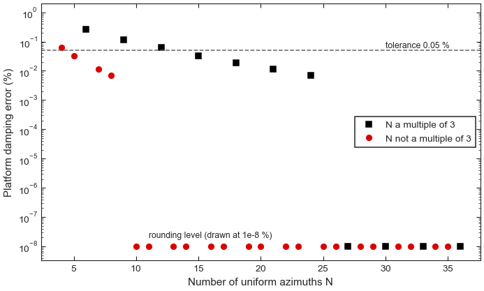
Worst-case damping error of the platform mode for a uniform average of N azimuths (pinned model). A count that is a multiple of 3 (squares) is first disturbed by the harmonic of order N; any other count (circles) only by the harmonic of order 3N.
Step by step
1. The blade-number rule. A uniform average of \(N\) samples cancels every
harmonic except the multiples of \(N\). After the MBC3 transform an isotropic
\(B\)-bladed rotor leaves content only at multiples of \(B\), so the first
order that survives the average is \(\operatorname{lcm}(N, B)\)
(first_alias_order()). For \(B = 3\),
12 azimuths are first disturbed by order 12, but 13 azimuths only by order 39. A count
that is not a multiple of the blade number is worth three times as many samples.
alias_free_azimuth_count() inverts the rule:
7 azimuths clear content up to order 18, and 10 clear content up to order 24, the
highest order of this model.
2. The reference. 72 uniform azimuths resolve every order up to 35, so their
average is exact for this model. locate_azimuth_state()
finds the azimuth position and rotor-speed states from their DOF_GeAz
descriptions. The reference has the platform pair, a fast rotor-speed root, and an
azimuth eigenvalue of \(-1.6\times10^{-4}\) 1/s that should be zero: the residue
of the averaging.
3. Pinning the azimuth direction. The azimuth column of \(\mathbf A(\psi)\) is
large and rich in high harmonics, and with the rotor-speed state it forms a nearly
defective pair. A coarse average of it can be badly wrong: the 9-azimuth mean of the
delivered matrices makes the platform mode unstable (+0.041 1/s). The orbit tangent of
the dense mean, azimuth_tangent(), is the direction along
the periodic orbit. pin_azimuth() modifies every sample so
that this direction is an exact null vector. Every average of the pinned samples then
has an exact zero eigenvalue, and all the other eigenvalues of the reference are
unchanged. The pinned 9-azimuth mean gives the platform mode at
\(-0.00965 \pm 0.30077j\), close to the reference.
4. The error of each azimuth count.
azimuth_count_table() evaluates the exact
eigenvalues of the uniform \(N\)-mean of the fitted harmonic model, worst over 24
start azimuths, and reports the damping and frequency error of each branch. The
figure shows the rule at work: every count that is not a multiple of 3 from 10 up is
exact to rounding, because its first alias lies above order 24, while 12, 18 and 24
azimuths, the customary choices, still carry errors of up to 0.06 % in damping and
0.6 % in frequency. recommended_resolved is the smallest count whose first alias
the samples resolve and whose error meets the tolerance: 5 azimuths for 0.05 %.
5. The error estimate of a real-looking linearization. OpenFAST takes each
snapshot at the first time step at or past its target azimuth, so the delivered grid
is uneven. The script builds 36 azimuths, each delayed by up to 30 % of the spacing.
estimate_averaging_error() reports three
terms per branch, in percent of the reference value:
sampling: the error of a coarser grid. Sub-grids of the delivered samples (18 and 9 azimuths here) are measured exactly; the column
fis the frequency error;quadrature: the arithmetic mean that the MBC3 transform applies against the interval-weighted mean of the uneven grid;
periodicity: the difference between the averaged eigenvalue and the Floquet exponent of the periodic model, from a second-order sideband estimate.
On the delivered samples the sampling errors are enormous (341 % and 585 % in damping)
and the quadrature error is 2.6 %: both come from the azimuth column. After pinning
they fall to 0.07 % and 0.4 % (sampling) and 0.005 % (quadrature). The branch is still
not accepted (accept is False): with the default tolerances of 1 % in damping
and 0.1 % in frequency, the frequency errors of 0.17 % and 1.0 % are too large.
Azimuth assessment: consistent means that the azimuth residual cannot move the
platform damping beyond the tolerance.
The last two lines show what no single grid can measure about itself: the uneven 36-azimuth mean puts the platform damping at \(0.010346/0.2985 = 3.46\,\%\), the dense mean at 3.21 %, a 7.7 % difference. The estimate assesses sub-grids and hypothetical grids against the samples you have; it cannot bound the error of the full delivered grid, which is why the commensurate time step of step 7 matters.
6. The check against Floquet theory. On the dense uniform grid the periodicity term
moves the averaged platform eigenvalue from \(-0.0096079 + 0.2992479j\) to
\(-0.0096090 + 0.2992057j\). The Floquet exponent computed independently from the
monodromy matrix over one revolution, monodromy_exponents()
with 720 azimuths, is \(-0.0096090 + 0.2992040j\). The sideband estimate recovers
the difference between the average and the periodic system to within
\(2\times10^{-6}\) 1/s.
7. A commensurate time step.
commensurate_time_step() suggests a time
step no larger than the one requested (0.025 s) that places every target azimuth on a
whole number of steps: 0.024933 s, seven steps per 10 degrees. With it, and the rotor
at its trimmed speed, the delivered grid is uniform, the quadrature term vanishes and
the uneven-grid error of step 5 does not arise.
Exercises
In
sample, passdecay=0.3toperiodic_rotor_matrixand rerun. The high harmonics are now smaller, so the errors of the multiples of 3 fall faster with N.Pass
grid=13toestimate_averaging_error: a hypothetical 13-azimuth grid has its first alias at order 39, above the 17 orders 36 azimuths resolve, so the status readsunresolvedand the branch is not accepted. A denser reference is needed to confirm such a count.
See Azimuth averaging for every option and Floquet analysis of the periodic system for the periodic theory. Next: Tutorial 6: State-space, Kalman and LPV export.