Tutorial 3: Mode identification and the Campbell diagram
Goal: label the modes of an operating point by their physics, track them across a
sweep with ModalPipeline, find where they cross the per-revolution
excitation lines, export the Campbell diagram as tables, and draw it.
Script: examples/03_mode_identification_campbell.py · Data: a synthetic
sweep of ten operating points, 4 to 15 m/s (see The synthetic turbine) ·
Run time: seconds
The code
from vane import ModalPipeline, discover_operating_points
from vane.export import campbell_table, resonance_table, write_table
from vane.io import mbc3_transform
from vane.modal import label_solution, modes_from_mbc
from vane.viz import plot_campbell, plot_campbell_static

WIND_SPEEDS = (4.0, 5.0, 6.0, 7.0, 8.0, 9.0, 10.0, 11.0, 13.0, 15.0)  # m/s
HARMONICS = (1, 3, 6)
def main(argv: list[str] | None = None) -> int:
    """Run the tutorial.

    Parameters
    ----------
    argv : list[str] or None, optional
        Command-line arguments; ``None`` reads ``sys.argv``.

    Returns
    -------
    int
        The exit status.
    """
    args = output_parser(__doc__).parse_args(argv)
    with output_directories(args.output) as (data, figures):
        # 1. Write the sweep: the .lin files of every wind speed, in one directory.
        turbine = SyntheticTurbine()
        turbine.write_sweep(data / "sweep", WIND_SPEEDS, n_azimuths=12)
        points = discover_operating_points(data / "sweep")
        print(f"Discovered {len(points)} operating points:")
        for point in points:
            first = point[0]
            print(
                f"  {point.name}: {len(point)} azimuths, wind {first.wind_speed:4.1f} "
                f"m/s, rotor {first.rotor_speed * 30 / np.pi:6.3f} rpm"
            )

        # 2. Physical labels at one operating point.
        at_8 = next(p for p in points if p.name == "ws080")
        solution = modes_from_mbc(mbc3_transform(at_8))
        print()
        print("Labels at 8 m/s")
        print("  f_n (Hz)  label                          category             conf.")
        for k, label in enumerate(label_solution(solution)):
            print(
                f"  {solution.natural_frequencies_hz[k]:8.4f}  {label.label:<30} "
                f"{label.category.name:<20} {label.confidence:5.2f}"
            )

        # 3. Track the points below rated on the rotor-speed axis.
        rated = turbine.rated_wind_speed
        below = [p for p in points if p[0].wind_speed <= rated + 0.5]
        pipeline = ModalPipeline(harmonics=HARMONICS)
        result = pipeline.run(below, parameter_name="rotor_speed_rpm")
        diagram = result.campbell
        rpm = np.asarray(diagram.parameter_values)
        print()
        print(f"Campbell diagram: {len(diagram.tracks)} tracks over {rpm.size} points")
        print(
            "  track  label                          f(first)  f(last)  conf.  ambig."
        )
        for index, track in enumerate(diagram.tracks):
            print(
                f"  {index:5d}  {track.label.label:<30} "
                f"{track.natural_frequencies_hz[0]:8.4f} "
                f"{track.natural_frequencies_hz[-1]:8.4f}  {track.confidence:5.2f}  "
                f"{track.is_ambiguous}"
            )
        print()
        print("Resonance crossings")
        print("  track  harmonic  rotor (rpm)  f (Hz)  damping  severity")
        for crossing in result.resonances:
            print(
                f"  {crossing.track_index:5d}  {crossing.harmonic:7d}P  "
                f"{crossing.rotor_speed_rpm:11.2f}  {crossing.frequency_hz:6.3f}  "
                f"{crossing.damping_ratio:7.4f}  {crossing.severity.value}"
            )

        # 4. Tables: CSV always, Excel when openpyxl is installed.
        tracks = campbell_table(diagram)
        crossings = resonance_table(result.resonances)
        write_table(tracks, data / "campbell.csv")
        write_table(crossings, data / "resonances.csv")
        print()
        print(f"Campbell table: {len(tracks)} rows, columns {list(tracks.columns)}")
        if importlib.util.find_spec("openpyxl") is not None:
            write_table(tracks, data / "campbell.xlsx")
            print("Tables written: campbell.csv, resonances.csv, campbell.xlsx")
        else:
            print(
                "Tables written: campbell.csv, resonances.csv (no openpyxl: no .xlsx)"
            )

        # 5. The interactive diagram (Plotly HTML) and a static one (Matplotlib).
        plot_campbell(diagram).write_html(data / "campbell.html")
        figure = plot_campbell_static(diagram, harmonics=HARMONICS, size="double")
        save_figure(figure, figures / "tutorial_campbell.png")

        # 6. Past rated the rotor speed is constant: use the wind-speed axis.
        print()
        try:
            pipeline.run(points, parameter_name="rotor_speed_rpm")
        except ValueError as error:
            print("Rotor-speed axis over the full sweep raises ValueError:")
            print(
                textwrap.fill(
                    str(error), width=86, initial_indent="  ", subsequent_indent="  "
                )
            )
        by_wind = pipeline.run(points, parameter_name="wind_speed")
        print(
            f"Wind-speed axis: {len(by_wind.campbell.tracks)} tracks over "
            f"{len(by_wind.campbell.parameter_values)} points, "
            f"{len(by_wind.resonances)} resonances reported"
        )
    return 0
Run it
$ python examples/03_mode_identification_campbell.py
Discovered 10 operating points:
  ws040: 12 azimuths, wind  4.0 m/s, rotor  4.578 rpm
  ws050: 12 azimuths, wind  5.0 m/s, rotor  5.722 rpm
  ws060: 12 azimuths, wind  6.0 m/s, rotor  6.866 rpm
  ws070: 12 azimuths, wind  7.0 m/s, rotor  8.011 rpm
  ws080: 12 azimuths, wind  8.0 m/s, rotor  9.155 rpm
  ws090: 12 azimuths, wind  9.0 m/s, rotor 10.300 rpm
  ws100: 12 azimuths, wind 10.0 m/s, rotor 11.444 rpm
  ws110: 12 azimuths, wind 11.0 m/s, rotor 12.100 rpm
  ws130: 12 azimuths, wind 13.0 m/s, rotor 12.100 rpm
  ws150: 12 azimuths, wind 15.0 m/s, rotor 12.100 rpm

Labels at 8 m/s
  f_n (Hz)  label                          category             conf.
    0.3000  1st Tower Side-Side            TOWER_SIDE_SIDE_1     0.99
    0.3215  1st Tower Fore-Aft             TOWER_FORE_AFT_1      0.98
    0.5564  1st Blade Flap (Regressive)    BLADE_FLAP_1          0.99
    0.7133  1st Blade Flap (Collective)    BLADE_FLAP_1          0.98
    0.8590  1st Blade Flap (Progressive)   BLADE_FLAP_1          1.00

Campbell diagram: 5 tracks over 8 points
  track  label                          f(first)  f(last)  conf.  ambig.
      0  1st Tower Side-Side              0.3001   0.2999   1.00  False
      1  1st Tower Fore-Aft               0.3213   0.3217   1.00  False
      2  1st Blade Flap (Regressive)      0.6117   0.5278   1.00  False
      3  1st Blade Flap (Collective)      0.6936   0.7324   1.00  False
      4  1st Blade Flap (Progressive)     0.7633   0.9270   1.00  False

Resonance crossings
  track  harmonic  rotor (rpm)  f (Hz)  damping  severity
      0        3P         6.00   0.300   0.0093  high
      1        3P         6.43   0.321   0.0488  medium
      2        3P        10.80   0.540   0.1555  low
      2        6P         5.94   0.594   0.1169  low
      3        6P         7.03   0.703   0.1015  low
      4        6P         8.43   0.843   0.0912  low

Campbell table: 40 rows, columns ['track', 'label', 'multiblade', 'rotor_speed_rpm', 'natural_frequency_hz', 'damping_ratio', 'confidence', 'is_ambiguous']
Tables written: campbell.csv, resonances.csv, campbell.xlsx
Figure written: tutorial_campbell.png

Rotor-speed axis over the full sweep raises ValueError:
  operating points must have distinct 'rotor_speed_rpm' values; got duplicates
  (12.099913703504432) in [4.577932783095278, 5.72193851403982, 6.865944244984365,
  8.010904905587461, 9.154910636532005, 10.2998712971351, 11.44387702807964,
  12.099913703504432, 12.099913703504432, 12.099913703504432]; use the wind-speed axis
  instead: parameter_name='wind_speed' (CLI: --parameter wind), which is distinct
  across these operating points
Wind-speed axis: 5 tracks over 10 points, 0 resonances reported
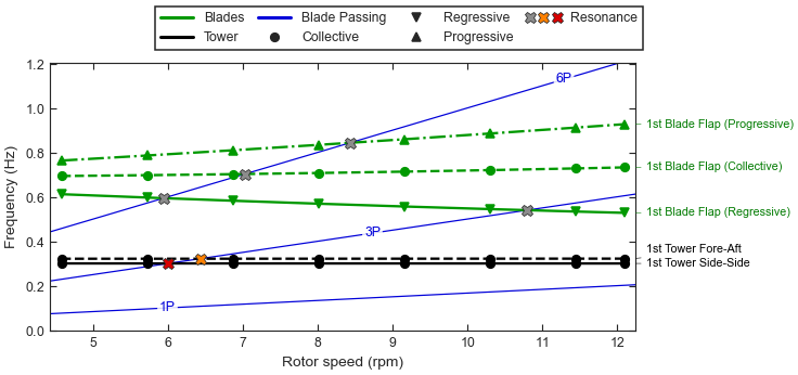
The five tracks against rotor speed, grouped by mode family, the 1P, 3P and 6P excitation lines (dashed, from the bottom), and the crossings coloured by severity. The flap triplet fans out with rotor speed; the tower modes cross 3P near 6 rpm and the regressive flap mode near 10.8 rpm.
Step by step
1. Discovering operating points. discover_operating_points() groups
the files of a directory by their <case> root, so ws080.1.lin to
ws080.12.lin form the operating point ws080. Each returned point is a sequence
of LinFile objects, ready for every function that takes
the files of one point. The sweep has eight points below rated, where the rotor speed
rises with the wind, and two above it at the rated 12.1 rpm.
2. Physical labels. label_solution() names each mode of
one operating point from the share of its participation carried by each kind of degree
of freedom, using left and right eigenvectors so the result does not depend on the
units of the states. The category is the winning
DofCategory; confidence is its share (0.98 to 1.00
here, since the synthetic modes are nearly pure). For the flap triplet the
multi-blade coordinates decide the type: equal cosine and sine parts whirling backward
make the regressive mode, forward the progressive one, and the collective coordinate
the collective mode.
3. Tracking and the Campbell diagram. ModalPipeline.run runs the MBC3 transform and the eigenanalysis of
Tutorial 2: MBC3 transform and eigenanalysis at every point, labels the modes, and links them from point to
point by their mode-shape correlation (MAC) and frequency continuity. Each
ModeTrack is one line of the diagram; its
confidence is the weakest link along the track and is_ambiguous flags a near
tie. Here every link is unambiguous. The regressive mode falls from 0.612 to 0.528 Hz
and the progressive mode rises from 0.763 to 0.927 Hz as the rotor speeds up: the
\(\mp\Omega\) split of Tutorial 2: MBC3 transform and eigenanalysis growing with \(\Omega\).
The points are tracked on the rotor-speed axis, the default
(parameter_name="rotor_speed_rpm"), because the resonance search needs it. The
script passes only the points up to 11 m/s, whose rotor speeds are all different.
4. Resonance crossings. A rotor turning at rpm excites the structure at
n * rpm / 60 Hz. ModalPipeline(harmonics=(1, 3, 6)) searches the 1P, 3P and 6P
lines (the default is (1, 3, 6, 9)), and result.resonances lists each crossing,
interpolated between operating points. Check the first by hand: the side-side mode at
0.300 Hz meets 3P where 3 * rpm / 60 = 0.300, at 6.00 rpm. The severity follows
the damping ratio at the crossing: below 0.01 is high (the side-side mode, with
almost no aerodynamic damping), 0.01 to 0.05 medium (the fore-aft mode) and above
low (the aerodynamically damped flap modes). No mode crosses 1P, which stays below
0.21 Hz.
5. Tables. campbell_table() flattens the diagram into a
pandas.DataFrame with one row per track and operating point (5 tracks x 8
points = 40 rows), and resonance_table() does the same for the
crossings. write_table() chooses the format from the suffix:
.csv, .json, .mat, or .xlsx when openpyxl is installed (the
excel extra). The script writes the Excel file only when openpyxl is
available.
6. Plots. plot_campbell() returns an interactive
Plotly figure with the damping ratio and confidence of each point on hover; the script
saves it as campbell.html. plot_campbell_static()
draws the same diagram with Matplotlib for reports, as in the figure above: the tracks
styled by mode family, the excitation lines of the chosen harmonics and the crossings.
For a diagram of your own, track_curve()
gives each track’s parameter values, frequencies and damping ratios, and
excitation_frequencies() the excitation lines.
7. Past rated, use the wind-speed axis. Above rated the trimmed rotor speed is
constant, so three points share 12.1 rpm and cannot be ordered by it. The pipeline
rejects that axis with the ValueError shown, rather than tracking modes between
points in an arbitrary order, and names the remedy. On the wind-speed axis
(parameter_name="wind_speed") all ten points are tracked. No crossings are reported
there, because the excitation lines are defined in rotor speed.
Exercises
Open
campbell.html(run with--output) and hover over a track to see its damping ratio and label confidence at each point.Change
HARMONICSto(1, 3, 6, 9). The 9P line crosses the collective and progressive flap modes at low rotor speed; check the first crossing by hand.Pass
ModalPipeline(branch_review=True)and confirm thatresult.identification.branch_groupsis empty: no two tracks of this turbine approach each other closely enough to be contested.
See Mode identification and Campbell diagrams for the options, and Mode identification and Campbell diagram, resonance, and uncertainty for the methods. Next: Tutorial 4: Mode shapes.